Optimizing Access Patterns#

Introduction#

In this page we will be showing how we can take an existing MDIO and add fast access, lossy, versions of the data in X/Y/Z cross-sections (slices).

We can re-use the MDIO dataset we created in the Quickstart page. Please run it first.

We will define our compression levels first. We will use this to adjust the quality of the lossy compression.

from enum import Enum

class MdioZfpQuality(float, Enum):
    """Config options for ZFP compression."""

    VERY_LOW = 6
    LOW = 3
    MEDIUM = 1
    HIGH = 0.1
    VERY_HIGH = 0.01
    ULTRA = 0.001

We will use the lower level MDIOAccessor to open the existing file in write mode that allows us to modify its raw metadata. This can be dangerous, we recommend using only provided tools to avoid data corruption.

We specify the original access pattern of the source data "012" with some parameters like caching. For the rechunking, we recommend using the single threaded "zarr" backend to avoid race conditions.

We also define a dict for common arguments in rechunking.

from mdio.api.accessor import MDIOAccessor

mdio_path = "filt_mig.mdio"

orig_mdio_cached = MDIOAccessor(
    mdio_path_or_buffer=mdio_path,
    mode="w",
    access_pattern="012",
    storage_options=None,
    return_metadata=False,
    new_chunks=None,
    backend="zarr",
    memory_cache_size=2**28,
    disk_cache=False,
)

Compression (Lossy)#

Now, let’s define our compression level. The compression ratios vary a lot on the data characteristics. However, the compression levels here are good guidelines that are based on standard deviation of the original data.

We use ZFP’s fixed accuracy mode with a tolerance based on data standard deviation, as mentioned above. For more ZFP options you can see its documentation.

Empirically, for this dataset, we see the following size reductions (per copy):

10 : 1 on VERY_LOW
7.5 : 1 on LOW
4.5 : 1 on MEDIUM
3 : 1 on HIGH
2 : 1 on VERY_HIGH
1.5 : 1 on ULTRA

from numcodecs import ZFPY
from zfpy import mode_fixed_accuracy

std = orig_mdio_cached.stats["std"]  # standard deviation of original data

quality = MdioZfpQuality.LOW
tolerance = quality * std
sample_compressor = ZFPY(mode_fixed_accuracy, tolerance=tolerance)

common_kwargs = {"overwrite": True, "compressor": sample_compressor}

Optimizing IL/XL/Z Independently#

In this cell, we will demonstrate how to create IL/XL and Z (two-way-time) optimized versions independently. In the next section we will do the same with the batch mode where the data only needs to be read into memory once.

In the example below, each rechunking operation will read the data from the original MDIO dataset and discard it. We did enable 256 MB (2^28 bytes) memory cache above, it will help some, but still not ideal.

from mdio.api.convenience import rechunk

rechunk(orig_mdio_cached, (4, 512, 512), suffix="fast_il", **common_kwargs)
rechunk(orig_mdio_cached, (512, 4, 512), suffix="fast_xl", **common_kwargs)
rechunk(orig_mdio_cached, (512, 512, 4), suffix="fast_z", **common_kwargs)

Rechunking to fast_il: 100%|██████████| 3/3 [00:01<00:00,  1.77chunk/s]
Rechunking to fast_xl: 100%|██████████| 3/3 [00:01<00:00,  1.90chunk/s]
Rechunking to fast_z: 100%|██████████| 3/3 [00:01<00:00,  1.97chunk/s]

We can now open the original MDIO dataset and the fast access patterns. When printing the chunks attribute, we see the original one first, and the subsequent ones show data is rechunked with ZFP compression.

from mdio import MDIOReader

orig_mdio = MDIOReader(mdio_path)
il_mdio = MDIOReader(mdio_path, access_pattern="fast_il")
xl_mdio = MDIOReader(mdio_path, access_pattern="fast_xl")
z_mdio = MDIOReader(mdio_path, access_pattern="fast_z")

print(orig_mdio.chunks, orig_mdio._traces.compressor)
print(il_mdio.chunks, il_mdio._traces.compressor)
print(xl_mdio.chunks, xl_mdio._traces.compressor)
print(z_mdio.chunks, z_mdio._traces.compressor)

(64, 64, 64) Blosc(cname='zstd', clevel=5, shuffle=SHUFFLE, blocksize=0)
(4, 187, 512) ZFPY(mode=4, tolerance=2.7916183359718256, rate=-1, precision=-1)
(345, 4, 512) ZFPY(mode=4, tolerance=2.7916183359718256, rate=-1, precision=-1)
(345, 187, 4) ZFPY(mode=4, tolerance=2.7916183359718256, rate=-1, precision=-1)

We can now compare the sizes of the compressed representations to original.

Below commands are for UNIX based operating systems and won’t work on Windows.

!du -hs {mdio_path}/data/chunked_012
!du -hs {mdio_path}/data/chunked_fast_il
!du -hs {mdio_path}/data/chunked_fast_xl
!du -hs {mdio_path}/data/chunked_fast_z

149M	filt_mig.mdio/data/chunked_012
 21M	filt_mig.mdio/data/chunked_fast_il
 20M	filt_mig.mdio/data/chunked_fast_xl
 21M	filt_mig.mdio/data/chunked_fast_z

Comparing local disk read speeds for inlines:

%timeit orig_mdio[175]  # 3d chunked
%timeit il_mdio[175]  # inline optimized

31.1 ms ± 825 µs per loop (mean ± std. dev. of 7 runs, 10 loops each)
3.6 ms ± 52.9 µs per loop (mean ± std. dev. of 7 runs, 100 loops each)

For crosslines:

%timeit orig_mdio[:, 90]  # 3d chunked
%timeit xl_mdio[:, 90]  # xline optimized

65.3 ms ± 705 µs per loop (mean ± std. dev. of 7 runs, 10 loops each)
8.76 ms ± 353 µs per loop (mean ± std. dev. of 7 runs, 100 loops each)

Finally, for Z (time-slices):

%timeit orig_mdio[..., 751]  # 3d chunked
%timeit z_mdio[..., 751]  # time-slice optimized

6.36 ms ± 185 µs per loop (mean ± std. dev. of 7 runs, 100 loops each)
872 µs ± 8.24 µs per loop (mean ± std. dev. of 7 runs, 1,000 loops each)

We can check the subjective quality of the compression by visually comparing two inlines. Similar to the example we had in the Compression page.

import matplotlib.pyplot as plt
from mpl_toolkits.axes_grid1 import make_axes_locatable

vmin = -3 * std
vmax = 3 * std

imshow_kw = dict(vmin=vmin, vmax=vmax, cmap="gray_r", interpolation="bilinear", aspect="auto")


def attach_colorbar(image, axis):
    divider = make_axes_locatable(axis)
    cax = divider.append_axes("top", size="2%", pad=0.05)
    plt.colorbar(image, cax=cax, orientation="horizontal")
    cax.xaxis.set_ticks_position("top")
    cax.tick_params(labelsize=8)


def plot_image_and_cbar(data, axis, title):
    image = axis.imshow(data.T, **imshow_kw)
    attach_colorbar(image, axis)
    axis.set_title(title, y=-0.15)


def plot_inlines_with_diff(orig, compressed, title):
    fig, ax = plt.subplots(1, 4, sharey="all", sharex="all", figsize=(8, 5))

    diff = orig[200] - compressed[200]

    plot_image_and_cbar(orig[200], ax[0], "original")
    plot_image_and_cbar(compressed[200], ax[1], "lossy")
    plot_image_and_cbar(diff, ax[2], "difference")
    plot_image_and_cbar(diff * 1_000, ax[3], "1,000x difference")

    plt.suptitle(f"{title} ({std=})")
    fig.tight_layout()

    plt.show()


plot_inlines_with_diff(orig_mdio, il_mdio, "")

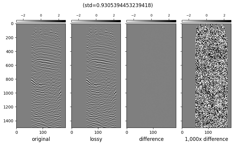
../_images/7208ae0d0a25d34cf19f7b930f958a35bed575037806e92b9a243375ff64928c.png

In conclusion, we show that by generating optimized, lossy compressed copies of the data for certain access patterns yield big performance benefits when reading the data.

The differences are orders of magnitude larger on big datasets and remote stores, given available network bandwidth.

Optimizing in Batch#

Now that we understand how rechunking and lossy compression works, we will demonstrate how to do this in batches.

The benefit of doing the batched processing is that the dataset gets read once. This is especially important if the original MDIO resides in a remote store like AWS S3, or Google Cloud’s GCS.

Note that we not are overwriting the old optimized chunks, just creating new ones with the suffix 2 to demonstrate we can create as many version of the original data as we want.

from mdio.api.convenience import rechunk_batch

rechunk_batch(
    orig_mdio_cached,
    chunks_list=[(4, 512, 512), (512, 4, 512), (512, 512, 4)],
    suffix_list=["fast_il2", "fast_xl2", "fast_z2"],
    **common_kwargs,
)

Rechunking to fast_il2,fast_xl2,fast_z2: 100%|██████████| 3/3 [00:05<00:00,  1.84s/chunk]

from mdio import MDIOReader

orig_mdio = MDIOReader(mdio_path)
il2_mdio = MDIOReader(mdio_path, access_pattern="fast_il2")
xl2_mdio = MDIOReader(mdio_path, access_pattern="fast_xl2")
z2_mdio = MDIOReader(mdio_path, access_pattern="fast_z2")

print(orig_mdio.chunks, orig_mdio._traces.compressor)
print(il_mdio.chunks, il2_mdio._traces.compressor)
print(xl_mdio.chunks, xl2_mdio._traces.compressor)
print(z_mdio.chunks, z2_mdio._traces.compressor)

(64, 64, 64) Blosc(cname='zstd', clevel=5, shuffle=SHUFFLE, blocksize=0)
(4, 187, 512) ZFPY(mode=4, tolerance=2.7916183359718256, rate=-1, precision=-1)
(345, 4, 512) ZFPY(mode=4, tolerance=2.7916183359718256, rate=-1, precision=-1)
(345, 187, 4) ZFPY(mode=4, tolerance=2.7916183359718256, rate=-1, precision=-1)