Get Started in 10 Minutes

In this page we will be showing basic capabilities of MDIO.

For demonstration purposes, we will download the Teapot Dome open-source dataset. The dataset details and licensing can be found at the SEG Wiki.

We are using the 3D seismic stack dataset named filt_mig.sgy.

The full link for the dataset (hosted on AWS): http://s3.amazonaws.com/teapot/filt_mig.sgy

Warning

For plotting, the notebook requires Matplotlib as a dependency. Please install it before executing using pip install matplotlib or conda install matplotlib.

Downloading the SEG-Y Dataset

Let’s download this dataset to our working directory. It may take from a few seconds up to a couple minutes based on your internet connection speed. The file is 386 MB in size.

The dataset is irregularly shaped, however it is padded to a rectangle with zero (dead traces). We will see that later at the live mask plotting.

from os import path
from urllib.request import urlretrieve

url = "http://s3.amazonaws.com/teapot/filt_mig.sgy"
urlretrieve(url, "filt_mig.sgy")

('filt_mig.sgy', <http.client.HTTPMessage at 0x1054e3620>)

Ingesting to MDIO

To do this, we can use the convenient SEG-Y to MDIO converter.

The inline and crossline values are located at bytes 181 and 185. Note that this doesn’t match any SEG-Y standards.

MDIO uses TGSAI/segy to parse the SEG-Y; the field names conform to its canonical keys defined in SEGY Binary Header Keys and SEGY Trace Header Keys. MDIO interprets the trace headers as SEG-Y Rev1 for historical reasons and will be more flexible in the next generation.

181 and 185 for Teapot should ideally map to cdp_x and cdp_y in the header arrays. However, because the file does not match the standard, they are mapped to the inline and crossline header keys on ingested headers.

In summary, we will use the byte locations as defined for ingestion. However, because inline / crossline and flipped with cdp_x / cdp_y, we must interchange the keys later.

from mdio import segy_to_mdio

segy_to_mdio(
    segy_path="filt_mig.sgy",
    mdio_path_or_buffer="filt_mig.mdio",
    index_bytes=(181, 185),
    index_names=("inline", "crossline"),
)

Scanning SEG-Y for geometry attributes: 100%|██████████| 7/7 [00:03<00:00,  1.89block/s]
Ingesting SEG-Y in 18 chunks: 100%|██████████| 18/18 [00:04<00:00,  4.12block/s]

It only took a few seconds to ingest, since this is a very small file.

However, MDIO scales up to TB (that’s ~1,000 GB) sized volumes!

Opening the Ingested MDIO File

Let’s open the MDIO file with the MDIOReader.

We will also turn on return_metadata function to get the live trace mask and trace headers.

from mdio import MDIOReader

mdio = MDIOReader("filt_mig.mdio", return_metadata=True)

Querying Metadata

Now let’s look at the Textual Header by the convenient text_header attribute.

You will notice the text header is parsed as a list of strings that are 80 characters long.

mdio.text_header

['C 1 CLIENT: ROCKY MOUNTAIN OILFIELD TESTING CENTER                              ',
 'C 2 PROJECT: NAVAL PETROLEUM RESERVE #3 (TEAPOT DOME); NATRONA COUNTY, WYOMING  ',
 'C 3 LINE: 3D                                                                    ',
 'C 4                                                                             ',
 'C 5 THIS IS THE FILTERED POST STACK MIGRATION                                   ',
 'C 6                                                                             ',
 'C 7 INLINE 1, XLINE 1:   X COORDINATE: 788937  Y COORDINATE: 938845             ',
 'C 8 INLINE 1, XLINE 188: X COORDINATE: 809501  Y COORDINATE: 939333             ',
 'C 9 INLINE 188, XLINE 1: X COORDINATE: 788039  Y COORDINATE: 976674             ',
 'C10 INLINE NUMBER:    MIN: 1  MAX: 345  TOTAL: 345                              ',
 'C11 CROSSLINE NUMBER: MIN: 1  MAX: 188  TOTAL: 188                              ',
 "C12 TOTAL NUMBER OF CDPS: 64860   BIN DIMENSION: 110' X 110'                    ",
 'C13                                                                             ',
 'C14                                                                             ',
 'C15                                                                             ',
 'C16                                                                             ',
 'C17                                                                             ',
 'C18                                                                             ',
 'C19 GENERAL SEGY INFORMATION                                                    ',
 'C20 RECORD LENGHT (MS): 3000                                                    ',
 'C21 SAMPLE RATE (MS): 2.0                                                       ',
 'C22 DATA FORMAT: 4 BYTE IBM FLOATING POINT                                      ',
 'C23 BYTES  13- 16: CROSSLINE NUMBER (TRACE)                                     ',
 'C24 BYTES  17- 20: INLINE NUMBER (LINE)                                         ',
 'C25 BYTES  81- 84: CDP_X COORD                                                  ',
 'C26 BYTES  85- 88: CDP_Y COORD                                                  ',
 'C27 BYTES 181-184: INLINE NUMBER (LINE)                                         ',
 'C28 BYTES 185-188: CROSSLINE NUMBER (TRACE)                                     ',
 'C29 BYTES 189-192: CDP_X COORD                                                  ',
 'C30 BYTES 193-196: CDP_Y COORD                                                  ',
 'C31                                                                             ',
 'C32                                                                             ',
 'C33                                                                             ',
 'C34                                                                             ',
 'C35                                                                             ',
 'C36 Processed by: Excel Geophysical Services, Inc.                              ',
 'C37               8301 East Prentice Ave. Ste. 402                              ',
 'C38               Englewood, Colorado 80111                                     ',
 'C39               (voice) 303.694.9629 (fax) 303.771.1646                       ',
 'C40 END EBCDIC                                                                  ']

MDIO parses the binary header into a Python dictionary.

We can easily query it by the binary_header attribute and see critical information about the original file.

mdio.binary_header

{'amp_recovery_code': 4,
 'aux_traces_per_ensemble': 0,
 'binary_gain_code': 1,
 'correlated_data_code': 2,
 'data_sample_format': 1,
 'data_traces_per_ensemble': 188,
 'ensemble_fold': 57,
 'extended_aux_traces_per_ensemble': 0,
 'extended_data_traces_per_ensemble': 0,
 'extended_ensemble_fold': 0,
 'extended_orig_samples_per_trace': 0,
 'extended_samples_per_trace': 0,
 'fixed_length_trace_flag': 0,
 'impulse_polarity_code': 1,
 'job_id': 9999,
 'line_num': 9999,
 'measurement_system_code': 2,
 'num_extended_text_headers': 0,
 'orig_sample_interval': 0,
 'orig_samples_per_trace': 1501,
 'reel_num': 1,
 'sample_interval': 2000,
 'samples_per_trace': 1501,
 'segy_revision': 0,
 'segy_revision_minor': 0,
 'sweep_freq_end': 0,
 'sweep_freq_start': 0,
 'sweep_length': 0,
 'sweep_taper_end': 0,
 'sweep_taper_start': 0,
 'sweep_trace_num': 0,
 'sweep_type_code': 0,
 'taper_type_code': 0,
 'trace_sorting_code': 4,
 'vertical_sum_code': 1,
 'vibratory_polarity_code': 0}

MDIO Grid, Dimensions, and Related Attributes

MDIO also has named dimensions, so we can see which dimension (axis) corresponds to which coordinate.

MDIO has an abstraction for an N-Dimensional grid. We can get the grid, and look at some of its properties.

mdio.grid.dim_names

('inline', 'crossline', 'sample')

mdio.grid.get_min("inline")

1

mdio.grid.get_max("crossline")

188

We can extract a dimension by name, and see its values.

The Dimension has name and coords that returns a string and a numpy array.

mdio.grid.select_dim("inline")

Dimension(coords=array([  1,   2,   3,   4,   5,   6,   7,   8,   9,  10,  11,  12,  13,
        14,  15,  16,  17,  18,  19,  20,  21,  22,  23,  24,  25,  26,
        27,  28,  29,  30,  31,  32,  33,  34,  35,  36,  37,  38,  39,
        40,  41,  42,  43,  44,  45,  46,  47,  48,  49,  50,  51,  52,
        53,  54,  55,  56,  57,  58,  59,  60,  61,  62,  63,  64,  65,
        66,  67,  68,  69,  70,  71,  72,  73,  74,  75,  76,  77,  78,
        79,  80,  81,  82,  83,  84,  85,  86,  87,  88,  89,  90,  91,
        92,  93,  94,  95,  96,  97,  98,  99, 100, 101, 102, 103, 104,
       105, 106, 107, 108, 109, 110, 111, 112, 113, 114, 115, 116, 117,
       118, 119, 120, 121, 122, 123, 124, 125, 126, 127, 128, 129, 130,
       131, 132, 133, 134, 135, 136, 137, 138, 139, 140, 141, 142, 143,
       144, 145, 146, 147, 148, 149, 150, 151, 152, 153, 154, 155, 156,
       157, 158, 159, 160, 161, 162, 163, 164, 165, 166, 167, 168, 169,
       170, 171, 172, 173, 174, 175, 176, 177, 178, 179, 180, 181, 182,
       183, 184, 185, 186, 187, 188, 189, 190, 191, 192, 193, 194, 195,
       196, 197, 198, 199, 200, 201, 202, 203, 204, 205, 206, 207, 208,
       209, 210, 211, 212, 213, 214, 215, 216, 217, 218, 219, 220, 221,
       222, 223, 224, 225, 226, 227, 228, 229, 230, 231, 232, 233, 234,
       235, 236, 237, 238, 239, 240, 241, 242, 243, 244, 245, 246, 247,
       248, 249, 250, 251, 252, 253, 254, 255, 256, 257, 258, 259, 260,
       261, 262, 263, 264, 265, 266, 267, 268, 269, 270, 271, 272, 273,
       274, 275, 276, 277, 278, 279, 280, 281, 282, 283, 284, 285, 286,
       287, 288, 289, 290, 291, 292, 293, 294, 295, 296, 297, 298, 299,
       300, 301, 302, 303, 304, 305, 306, 307, 308, 309, 310, 311, 312,
       313, 314, 315, 316, 317, 318, 319, 320, 321, 322, 323, 324, 325,
       326, 327, 328, 329, 330, 331, 332, 333, 334, 335, 336, 337, 338,
       339, 340, 341, 342, 343, 344, 345]), name='inline')

Fetching Data and Plotting

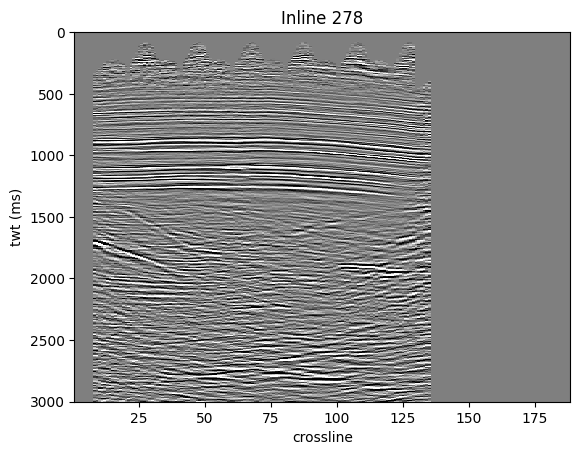
Now we will demonstrate getting an inline from MDIO.

Because MDIO can hold various dimensionality of data, we have to first query the inline location.

Then we can use the queried index to get the data itself.

We will also plot the inline, for this we need the crossline and sample coordinates.

MDIO stores dataset statistics. We can use the standard deviation (std) value of the dataset to adjust the gain.

import matplotlib.pyplot as plt


crosslines = mdio.grid.select_dim("crossline").coords
times = mdio.grid.select_dim("sample").coords

std = mdio.stats["std"]

inline_index = mdio.coord_to_index(278, dimensions="inline").item()
il_mask, il_headers, il_data = mdio[inline_index]

vmin, vmax = -2 * std, 2 * std
plt.pcolormesh(crosslines, times, il_data.T, vmin=vmin, vmax=vmax, cmap="gray_r")
plt.gca().invert_yaxis()
plt.title(f"Inline {278}")
plt.xlabel("crossline")
plt.ylabel("twt (ms)");

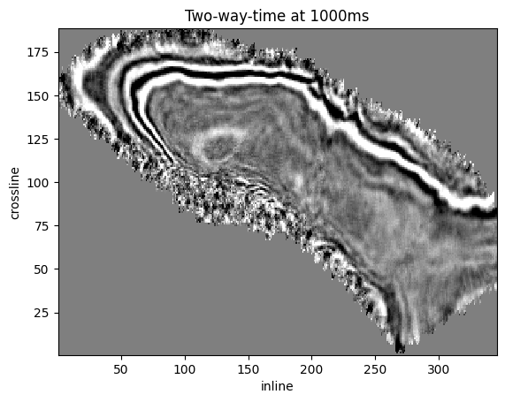
Let’s do the same with a time sample.

We already have crossline labels and standard deviation, so we don’t have to fetch it again.

We will display two-way-time at 1,000 ms.

inlines = mdio.grid.select_dim("inline").coords

twt_index = mdio.coord_to_index(1_000, dimensions="sample").item()
z_mask, z_headers, z_data = mdio[:, :, twt_index]

vmin, vmax = -2 * std, 2 * std
plt.pcolormesh(inlines, crosslines, z_data.T, vmin=vmin, vmax=vmax, cmap="gray_r")
plt.title(f"Two-way-time at {1000}ms")
plt.xlabel("inline")
plt.ylabel("crossline");

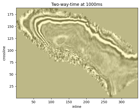
We can also overlay live mask with the time slice. However, in this example dataset is zero padded.

The live mask will always show True.

live_mask = mdio.live_mask[:]

plt.pcolormesh(inlines, crosslines, live_mask.T, vmin=0, vmax=1, alpha=0.5)
plt.pcolormesh(inlines, crosslines, z_data.T, vmin=vmin, vmax=vmax, cmap="gray_r", alpha=0.5)
plt.title(f"Two-way-time at {1000}ms")
plt.xlabel("inline")
plt.ylabel("crossline");

Query Headers

We can query headers for the whole dataset very quickly because they are separated from the seismic wavefield.

Let’s get all the headers for X and Y coordinates in this dataset.

As mentioned before, X Coordinates map to inline and Y Coordinates map to crossline due to non-standard Teapot data.

Note that the header maps will still honor the geometry/grid of the dataset!

mdio._headers[:]["inline"]  # actually cdp_x

array([[788937, 789047, 789157, ..., 809282, 809392, 809502],
       [788935, 789045, 789155, ..., 809279, 809389, 809499],
       [788932, 789042, 789152, ..., 809276, 809386, 809496],
       ...,
       [788044, 788154, 788264, ..., 808389, 808499, 808609],
       [788042, 788152, 788262, ..., 808386, 808496, 808606],
       [788039, 788149, 788259, ..., 808383, 808493, 808603]], dtype=int32)

mdio._headers[:]["crossline"]  # actually cdp_y

array([[938846, 938848, 938851, ..., 939329, 939331, 939334],
       [938956, 938958, 938961, ..., 939439, 939441, 939444],
       [939066, 939068, 939071, ..., 939549, 939551, 939554],
       ...,
       [976455, 976458, 976460, ..., 976938, 976941, 976943],
       [976565, 976568, 976570, ..., 977048, 977051, 977053],
       [976675, 976678, 976680, ..., 977158, 977161, 977163]], dtype=int32)

or both at he same time:

mdio._headers[:][["inline", "crossline"]]  # actually cdp_x, cdp_y

array([[(788937, 938846), (789047, 938848), (789157, 938851), ...,
        (809282, 939329), (809392, 939331), (809502, 939334)],
       [(788935, 938956), (789045, 938958), (789155, 938961), ...,
        (809279, 939439), (809389, 939441), (809499, 939444)],
       [(788932, 939066), (789042, 939068), (789152, 939071), ...,
        (809276, 939549), (809386, 939551), (809496, 939554)],
       ...,
       [(788044, 976455), (788154, 976458), (788264, 976460), ...,
        (808389, 976938), (808499, 976941), (808609, 976943)],
       [(788042, 976565), (788152, 976568), (788262, 976570), ...,
        (808386, 977048), (808496, 977051), (808606, 977053)],
       [(788039, 976675), (788149, 976678), (788259, 976680), ...,
        (808383, 977158), (808493, 977161), (808603, 977163)]],
      dtype={'names': ['inline', 'crossline'], 'formats': ['<i4', '<i4'], 'offsets': [188, 192], 'itemsize': 240})

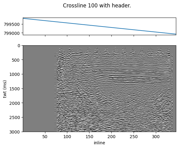
As we mentioned before, we can also get specific slices of headers while fetching a slice.

Let’s fetch a crossline, we are still using some previous parameters.

Since crossline is our second dimension, we can put the index in the second mdio[...] axis.

Since MDIO returns the headers as well, we can plot the headers on top of the image.

All headers will be returned, so we can select the X-coordinate with key inline.

Full headers can be mapped and plotted as well, but we won’t demonstrate that here.

crossline_index = mdio.coord_to_index(100, dimensions="crossline").item()
xl_mask, xl_headers, xl_data = mdio[:, crossline_index]

vmin, vmax = -2 * std, 2 * std

gs_kw = dict(height_ratios=(1, 5))
fig, ax = plt.subplots(2, 1, gridspec_kw=gs_kw, sharex="all")

ax[0].plot(inlines, xl_headers["inline"])

ax[1].pcolormesh(inlines, times, xl_data.T, vmin=vmin, vmax=vmax, cmap="gray_r")
ax[1].invert_yaxis()
ax[1].set_xlabel("inline")
ax[1].set_ylabel("twt (ms)")

plt.suptitle(f"Crossline {100} with header.");

MDIO to SEG-Y Conversion

Finally, let’s demonstrate going back to SEG-Y.

We will use the convenient mdio_to_segy function and write it out as a round-trip file.

from mdio import mdio_to_segy

mdio_to_segy(
    mdio_path_or_buffer="filt_mig.mdio",
    output_segy_path="filt_mig_roundtrip.sgy",
)

Array shape is (345, 188, 1501)
Setting (dask) chunks from (64, 64, 64) to (256, 188, 1501)

Unwrapping MDIO Blocks: 100%|██████████| 13/13 [00:01<00:00,  8.05it/s]
Merging lines: 100%|██████████| 345/345 [00:00<00:00, 1260.89it/s]

Validate Round-Trip SEG-Y File

We can validate if the round-trip SEG-Y file is matching the original using TGSAI/segy.

Step by step:

• Open original file

• Open round-trip file

• Compare text headers

• Compare binary headers

• Compare 100 random headers and traces

import numpy as np
from segy import SegyFile

original_segy = SegyFile("filt_mig.sgy")
roundtrip_segy = SegyFile("filt_mig_roundtrip.sgy")

# Compare text header
assert original_segy.text_header == roundtrip_segy.text_header

# Compare bin header
assert original_segy.binary_header == roundtrip_segy.binary_header

# Compare 100 random trace headers and traces
rng = np.random.default_rng()
rand_indices = rng.integers(low=0, high=original_segy.num_traces, size=100)
for idx in rand_indices:
    np.testing.assert_equal(original_segy.trace[idx], roundtrip_segy.trace[idx])