Seismic Data Compression

Altay Sansal

May 20, 2025

4 min read

In this page we will be showing compression performance of MDIO.

For demonstration purposes, we will use one of the Volve dataset stacks. The dataset is licensed by Equinor and Volve License Partners under Equinor Open Data Licence. License document and further information can be found here.

We are using the 3D seismic stack dataset named ST10010ZC11_PZ_PSDM_KIRCH_FAR_D.MIG_FIN.POST_STACK.3D.JS-017536.segy.

However, for convenience, we renamed it to volve.segy.

Warning

The examples below need the following extra dependencies:

1. Matplotlib for plotting.

2. Scikit-image for calculating metrics.

Please install them before executing using pip or conda.

Note

Even though we demonstrate with Volve here, this notebook can be run with any seismic dataset.

If you are new to MDIO we recommend you first look at our quick start guide

from mdio import MDIOReader
from mdio import segy_to_mdio

Ingestion

We will ingest three files:

1. Lossless mode

2. Lossy mode (with default tolerance)

3. Lossy mode (with more compression, more relaxed tolerance)

Lossless (Default)

segy_to_mdio(
    "volve.segy",
    "volve.mdio",
    (189, 193),
    # lossless=True,
    # compression_tolerance=0.01,
)

print("Done.")

Done.

Lossy Default

Equivalent to tolerance = 0.01.

segy_to_mdio(
    "volve.segy",
    "volve_lossy.mdio",
    (189, 193),
    lossless=False,
    # compression_tolerance=0.01,
)

print("Done.")

Done.

Lossy+ (A Lot of Compression)

Here we set tolerance = 1. This means all our errors will be comfortably under 1.0.

segy_to_mdio(
    "volve.segy",
    "volve_lossy_plus.mdio",
    (189, 193),
    lossless=False,
    compression_tolerance=1,
)

print("Done.")

Done.

Observe Sizes

Since MDIO uses a hierarchical directory structure, we provide a convenience function to get size of it using directory recursion and getting size.

from pathlib import Path


def get_dir_size(path: Path) -> int:
    """Get size of a directory recursively."""
    total = 0
    for entry in path.iterdir():
        if entry.is_file():
            total += entry.stat().st_size
        elif entry.is_dir():
            total += get_dir_size(entry)
    return total


def get_size(path: Path) -> int:
    """Get size of a folder or a file."""
    if path.is_file():
        return path.stat().st_size
    if path.is_dir():
        return get_dir_size(path)
    return 0  # Handle case where path is neither file nor directory


print(f"SEG-Y:\t{get_size('volve.segy') / 1024 / 1024:.2f} MB")
print(f"MDIO:\t{get_size('volve.mdio') / 1024 / 1024:.2f} MB")
print(f"Lossy:\t{get_size('volve_lossy.mdio') / 1024 / 1024:.2f} MB")
print(f"Lossy+:\t{get_size('volve_lossy_plus.mdio') / 1024 / 1024:.2f} MB")

SEG-Y:	1305.02 MB
MDIO:	998.80 MB
Lossy:	263.57 MB
Lossy+:	52.75 MB

Open Files, and Get Raw Statistics

lossless = MDIOReader("volve.mdio")
lossy = MDIOReader("volve_lossy.mdio")
lossy_plus = MDIOReader("volve_lossy_plus.mdio")

stats = lossless.stats
std = stats["std"]
min_ = stats["min"]
max_ = stats["max"]

Plot Images with Differences

Let’s define some plotting functions for convenience.

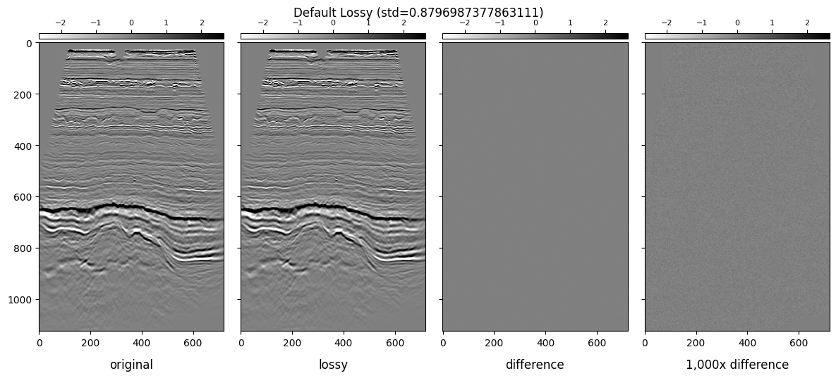
Here, we will make two plots showing data for lossy and lossy+ versions.

We will be showing the following subplots for each dataset:

1. Lossless Inline

2. Lossy Inline

3. Difference

4. 1,000x Gained Difference

We will be using ± 3 * standard_deviation of the colorbar ranges.

import matplotlib.pyplot as plt
from matplotlib.axes import Axes
from matplotlib.image import AxesImage
from mpl_toolkits.axes_grid1 import make_axes_locatable
from numpy.typing import NDArray

vmin = -3 * std
vmax = 3 * std

imshow_kw = {"vmin": -3 * std, "vmax": 3 * std, "cmap": "gray_r", "interpolation": "bilinear"}


def attach_colorbar(image: AxesImage, axis: Axes) -> None:
    """Attach a colorbar to an axis."""
    divider = make_axes_locatable(axis)
    cax = divider.append_axes("top", size="2%", pad=0.05)
    plt.colorbar(image, cax=cax, orientation="horizontal")
    cax.xaxis.set_ticks_position("top")
    cax.tick_params(labelsize=8)


def plot_image_and_cbar(data: NDArray, axis: Axes, title: str) -> None:
    """Plot an image with a colorbar."""
    image = axis.imshow(data.T, **imshow_kw)
    attach_colorbar(image, axis)
    axis.set_title(title, y=-0.15)


def plot_inlines_with_diff(orig: NDArray, compressed: NDArray, title: str) -> None:
    """Plot lossless and lossy inline with their differences."""
    fig, ax = plt.subplots(1, 4, sharey="all", sharex="all", figsize=(12, 5))

    diff = orig[200] - compressed[200]

    plot_image_and_cbar(orig[200], ax[0], "original")
    plot_image_and_cbar(compressed[200], ax[1], "lossy")
    plot_image_and_cbar(diff, ax[2], "difference")
    plot_image_and_cbar(diff * 1_000, ax[3], "1,000x difference")

    plt.suptitle(f"{title} ({std=})")
    fig.tight_layout()

    plt.show()


plot_inlines_with_diff(lossless, lossy, "Default Lossy")
plot_inlines_with_diff(lossless, lossy_plus, "More Lossy")

Calculate Metrics

For image quality, there are some metrics used by the broader image compression community.

In this example we will be using the following four metrics as comparison.

1. PSNR: Peak signal-to-noise ratio for an image. (higher is better)

2. SSIM: Mean structural similarity index between two images. (higher is better, maximum value is 1.0)

3. MSE: Compute the mean-squared error between two images. (lower is better)

4. NRMSE: Normalized root mean-squared error between two images. (lower is better)

For PSNR or SSIM, we use the global dataset range (max - min) as the normalization method.

In image compression community, a PSNR value above 60 dB (decibels) is considered acceptable.

We calculate these metrics on the same inline we show above.

from numpy.typing import NDArray
from skimage.metrics import mean_squared_error
from skimage.metrics import normalized_root_mse
from skimage.metrics import peak_signal_noise_ratio
from skimage.metrics import structural_similarity


def get_metrics(image_true: NDArray, image_test: NDArray) -> tuple[float, float, float, float]:
    """Get four image quality metrics."""
    psnr = peak_signal_noise_ratio(image_true[200], image_test[200], data_range=max_ - min_)
    ssim = structural_similarity(image_true[200], image_test[200], data_range=max_ - min_)
    mse = mean_squared_error(image_true[200], image_test[200])
    nrmse = normalized_root_mse(image_true[200], image_test[200])

    return psnr, ssim, mse, nrmse


print("Lossy", get_metrics(lossless, lossy))
print("Lossy+", get_metrics(lossless, lossy_plus))

Lossy (106.69280984265322, 0.9999999784224242, 9.176027503792131e-08, 0.000330489434736117)
Lossy+ (66.27609586061718, 0.999721336954417, 0.0010100110026414078, 0.0346731484815586)